Seismic Refraction Surveying

Applied Seismology

Earthquake Seismology

Recordings of distant or local earthquakes are used to infer earth structure and faulting characteristics.

Applied Seismology

A signal, similar to a sound pulse, is transmitted into the Earth. The signal recorded at the surface can be used to infer subsurface properties. There are two main classes of survey:

• Seismic Refraction: the signal returns to the surface by refraction at subsurface interfaces, and is recorded at distances much greater than depth of investigation.

• Seismic Reflection: the seismic signal is reflected back to the surface at layer interfaces, and is recorded at distances less than depth of investigation.

History of Seismology

Exploration seismic methods developed from early work on earthquakes:

• 1846: Irish physicist, Robert Mallett, makes first use of an artificial source in a seismic experiment.

• 1888: August Schmidt uses travel time vs. distance plots to determine subsurface seismic velocities.

• 1899: G.K. Knott explained refraction and reflection of seismic waves at plane boundaries.

• 1910: A. Mohorovicic identifies separate P and S waves on traveltime plots of distant earthquakes, and associates them with base of the crust, the Moho.

• 1916: Seismic refraction developed to locate artillery guns by measurement of recoil.

• 1921: ‘Seismos’ company founded to use seismic refraction to map salt domes, often associated with hydrocarbon traps.

• 1920: Practical seismic reflection methods developed. Within 10 years, the dominant method of hydrocarbon exploration.

Applications

Seismic Refraction

• Rock competence for engineering applications
• Depth to Bedrock
• Groundwater exploration
• Correction of lateral, near-surface, variations in seismic reflection surveys
• Crustal structure and tectonics

Seismic Reflection

• Detection of subsurface cavities
• Shallow stratigraphy
• Site surveys for offshore installations
• Hydrocarbon exploration
• Crustal structure and tectonics

Stress and Strain

A force applied to the surface of a solid body creates internal forces within the body:

• Stress is the ratio of applied force F to the area across which it is acts.

• Strain is the deformation caused in the body, and is expressed as the ratio of change in length (or volume) to original length (or volume).

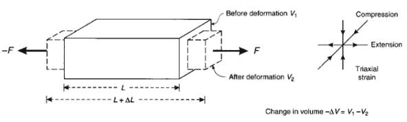
Triaxial Stress

Stresses act along three orthogonal axes, perpendicular to faces of solid, e.g. stretching a bar:

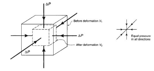
Pressure

Forces act equally in all directions perpendicular to faces of body, e.g. pressure on a cube in water:

Strain Associated with Seismic Waves

Inside a uniform solid, two types of strain can propagate as waves:

Axial Stress

Stresses act in one direction only, e.g. if sides of bar fixed:

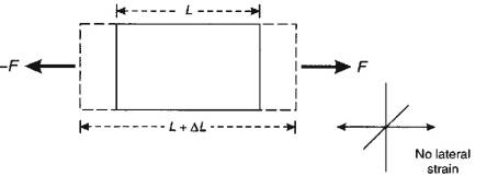
• Change in volume of solid occurs.
• Associated with P wave propagation

Shear Stress

Stresses act parallel to face of solid, e.g. pushing along a table:

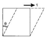
• No change in volume.
• Fluids such as water and air cannot support shear stresses.
• Associated with S wave propagation.

Hooke’s Law

Hooke’s Law essentially states that stress is proportional to strain.

• At low to moderate strains: Hooke’s Law applies and a solid body is said to behave elastically, i.e. will return to original form when stress removed.

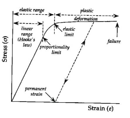
• At high strains: the elastic limit is exceeded and a body deforms in a plastic or ductile manner: it is unable to return to its original shape, being permanently strained, or damaged.

• At very high strains: a solid will fracture, e.g. in earthquake faulting.

Constant of proportionality is called the modulus, and is ratio of stress to strain, e.g. Young’s modulus in triaxial strain.

Seismic Body Waves

Seismic waves are pulses of strain energy that propagate in a solid. Two types of seismic wave can exist inside a uniform solid:

A) P waves (Primary, Compressional, Push-Pull)

Motion of particles in the solid is in direction of wave propagation.

• P waves have highest speed.
• Volumetric change
• Sound is an example of a P wave.

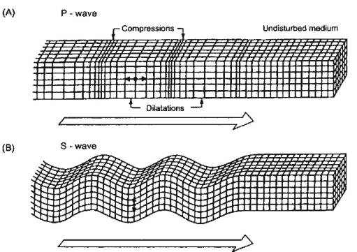
B) S waves (Secondary, Shear, Shake)

Particle motion is in plane perpendicular to direction of propagation.

• If particle motion along a line in perpendicular plane, then S wave is said to be plane polarised: SV in vertical plane, SH horizontal.
• No volume change
• S waves cannot exist in fluids like water or air, because the fluid is unable to support shear stresses.

Seismic Surface Waves

No stresses act on the Earth's surface (Free surface), and two types of surface wave can exist

A) Rayleigh waves

• Propagate along the surface of Earth
• Amplitude decreases exponentially with depth.
• Near the surface the particle motion is retrograde elliptical.
• Rayleigh wave speed is slightly less than S wave: ~92% V_S.

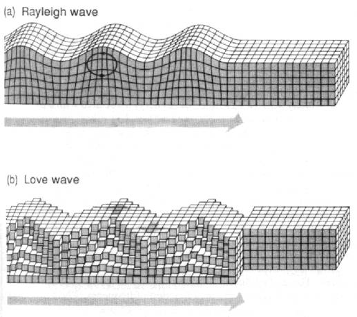
B. Love waves

Occur when a free surface and a deeper interface are present, and the shear wave velocity is lower in the top layer.

• Particle motion is SH, i.e. transverse horizontal
• Dispersive propagation: different frequencies travel at different velocities, but usually faster than Rayleigh waves.

Seismic Wave Velocities

The speed of seismic waves is related to the elastic properties of solid, i.e. how easy it is to strain the rock for a given stress.

• Depends on density, shear modulus, and axial modulus

Speed of wave propagation is NOT speed at which particles move in solid ( ~ 0.01 m/s ).

Constraints on Seismic Velocity

Seismic velocities vary with mineral content, lithology, porosity, pore fluid saturation, pore pressure, and to some extent temperature.

Igneous/Metamorphic Rocks

In igneous rocks with minimal porosity, seismic velocity increases with increasing mafic mineral content.

Sedimentary Rocks

In sedimentary rocks, effects of porosity and grain cementation are more important, and seismic velocity relationships are complex.

Various empirical relationships have been estimated from either measurements on cores or field observations:

1) P wave velocity as function of age and depth

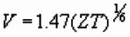km/s

where Z is depth in km and T is geological age in millions of years (Faust, 1951).

2) Time-average equation

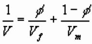
where f is porosity, V_f and V_m are P wave velocities of pore fluid and rock matrix respectively (Wyllie, 1958).

• Usually V_f ≈ 1500 m/s, while V_m depends on lithology.

• If the velocities of pore fluid and matrix known, then porosity can be estimated from the measured P wave velocity.

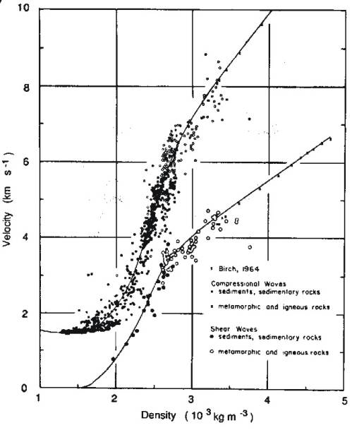
Nafe-Drake Curve

An important empirical relation exists between P wave velocity and density.

• Crossplotting velocity and density values of crustal rocks gives the Nafe-Drake curve after its discoverers.

• Only a few rocks such as salt (unusually low density) and sulphide ores (unusually high densities) lie off the curve.

Waves and Rays

In a homogeneous, isotropic medium, a seismic wave propagates away from its source at the same speed in every direction.

• The wavefront is the leading edge of the disturbance.
• The ray is the normal to the wavefront.

Huygen’s Principle

Every point on a wavefront can be considered a secondary source of spherical waves, and the position of the wavefront after a given time is the envelope of these secondary wavefronts.

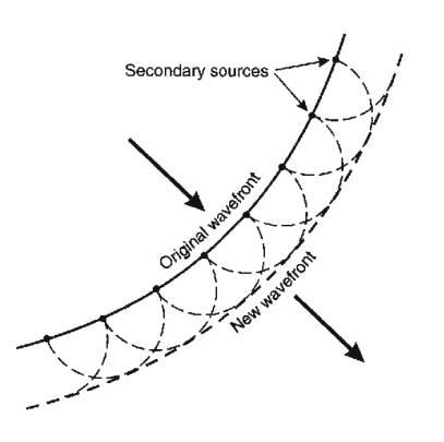
• Huygen’s construction can be used to explain reflection, refraction and diffraction of waves

• However, it is often simpler to consider wave propagation in terms of rays, though they cannot explain some effects such as diffraction into shadow zones.

Reflection and Refraction at Oblique Incidence

When a P wave is incident on a boundary, at which elastic properties change, two reflected waves (one P, one S) and two transmitted waves (one P, one S) are generated.

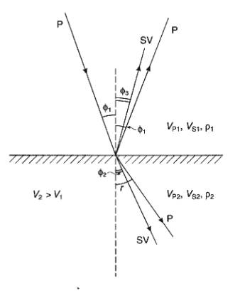
Angles of transmission and reflection of the S waves are less than the P waves.

Snell’s Law

Exact angles of transmission and reflection are given by:

p is known as the ray parameter.

Critical Angles

There are two critical angles corresponding to when transmitted P and S waves emerge at 90°.

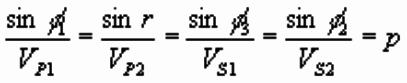
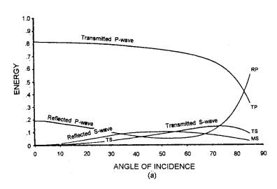
Amplitude of Reflected and Transmitted Waves

At oblique incidence, energy transformed between P and S waves at an interface.

Amplitudes of reflected and transmitted waves vary with angle of incidence in a complicated wave given by Zoeppritz equations.

Example

P wave reflection amplitude can increase at top of gas sand.

Wave Incident on Low Velocity Layer (No critical point)

Wave Incident on High Velocity Layer (P and S critical point)

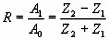
Normal Incidence Reflection Amplitudes

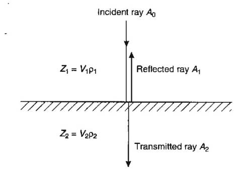
When angle of incidence is zero, amplitudes of reflected and transmitted waves simplify to the expressions below.

Reflection Coefficient:

Transmission Coefficient:

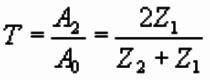
where Z is the acoustic (P wave) impedance of the layer, and is given by Z = Vr, where V is the P wave velocity and r the density.

• Same formulae apply to S waves at normal incidence.

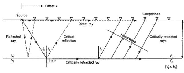
Critical Refraction

When seismic velocity increases at an interface (V₂>V₁), and the angle of incidence is increased from zero, the transmitted P wave will eventually emerge at 90°.

• Refracted wave travels along the upper boundary of the lower medium.

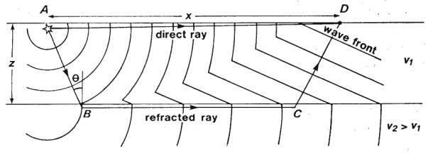
Head Waves

The interaction of this wave with the interface produces secondary sources that produce an upgoing wavefront, known as a head wave, by Huygen’s principle.

The ray associated with this head wave emerges from the interface at the critical angle.

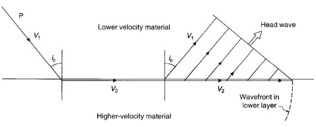
This phenomenon is the basis of the refraction surveying method.

Diffractions

Reflection by Huygen’s Principle

When a plane wavefront is incident on a plane boundary, each point of the boundary acts as a secondary source. The superposition of these secondary waves creates the reflection.

Diffraction by Huygen’s Principle

If interface truncates abruptly, then secondary waves do not cancel at the edge, and a diffraction is observed.

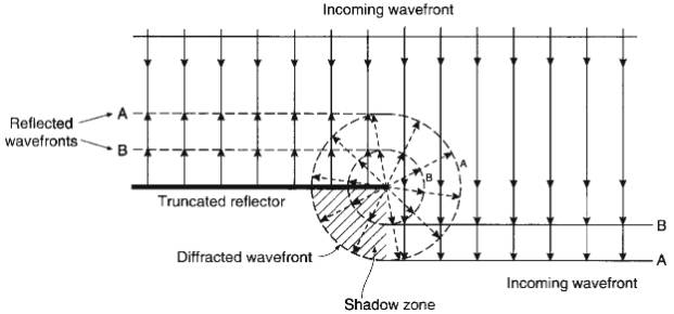
• This explains how energy can propagate into shadow zones.

• A small scattering object in the subsurface such as a boulder will produce a single diffraction.

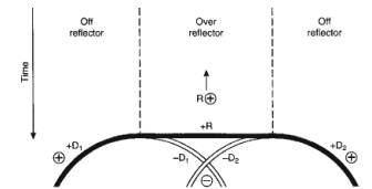
• A finite-length interface will produce diffractions from each end, and the interior parts of the arrivals will be opposite polarity.

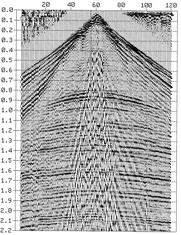
Seismic Field Record

Dynamite shot recorded using a 120-channel recording spread

Seismic Refraction Surveying

Refraction surveys use the process of critical refraction to infer interface depths and layer velocities.

Critical refraction requires an increase in velocity with depth. If not, then there is no critical; refraction: Hidden layer problem.

• Geophones laid out in a line to record arrivals from a shot. Recording at each geophone is a waveform called a seismogram.

• Direct signal from shot travels along top of first layer.

• Critical refraction is also recorded at distance beyond which angle of incidence becomes critical.

Example

For a shallow survey, 12-24 vertical 30 Hz geophones would be laid out to record a hammer or shotgun shot.

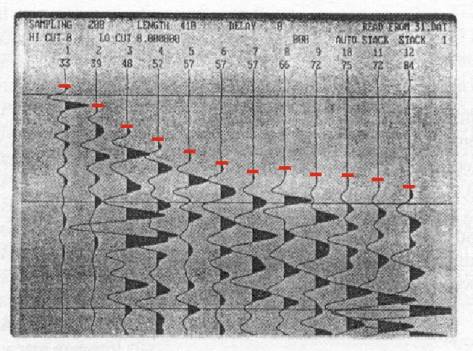
First Arrival Picking

In most refraction analysis, we only use the travel times of the first arrival on each recorded seismogram.

As velocity increases at an interface, critical refraction will become first arrival at some source-receiver offset.

First Break Picking

The onset of the first seismic wave, the first break, on each seismogram is identified and its arrival time picked.

Example of first break picking on Strataview field monitor

Travel Time Curves

Analysis of seismic refraction data is primarily based on interpretation of critical refraction travel times.

Plots of seismic arrival times vs. source-receiver offset are called travel time curves.

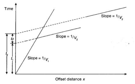
Example

Travel time curves for three arrivals shown previously:

• Direct arrival from source to receiver in top layer
• Critical refraction along top of second layer
• Reflection from top of second layer

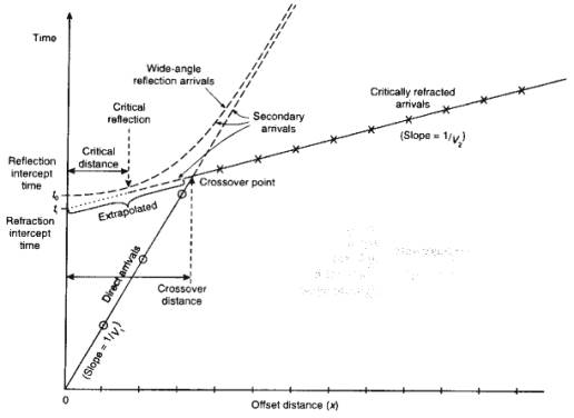
Critical Distance

Offset at which critical refraction first appears.

• Critical refraction has same travel time as reflection
• Angle of reflection same as critical angle

Crossover Distance

Offset at which critical refraction becomes first arrival.

Field Surveying

Usually we analyse P wave refraction data, but S wave data occasionally recorded

Land Surveys

Typically 12 or 24 geophones are laid out to record a shot along a cable, with takeouts to which geophones can be connected.

• Geophones and cable comprise a spread.
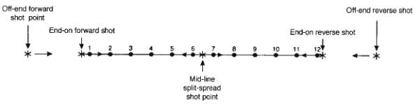
• Shot would usually be placed at one end of spread for first recording, then second recording made at other end.
• Off-end and split-spread shooting also possible.

Marine Surveys

Shot firing and seismograph recording systems are housed on a boat.

Two options for receivers:

A) Bottom-cable:

• Hydrophones contained in a ~55 m cable which is deployed or dragged along bottom of river or seabed.

B) Sonobouys

• Hydrophone is suspended from floating buoy containing radio telemetry to transmit seismogram to boat.
• Boat steams away from sonobouy firing an airgun.

Interpretation of Refraction Traveltime Data

After completion of a refraction survey first arrival times are picked from seismograms and plotted as traveltime curves

Interpretation objective is to infer interface depths and layer velocities

Data interpretation requires making assumption about layering in subsurface: look at shape and number of different first arrivals.

Assumptions

• Subsurface composed of stack of layers, usually separated by plane interfaces
• Seismic velocity is uniform in each layer
• Layer velocities increase in depth
• All ray paths are located in vertical plane, i.e. no 3-D effects with layers dipping out of plane of profile

Analysis based on considering critical refraction raypaths through subsurface.

[There are more sophisticated approaches to handle non-uniform velocity and 3-D layering.]

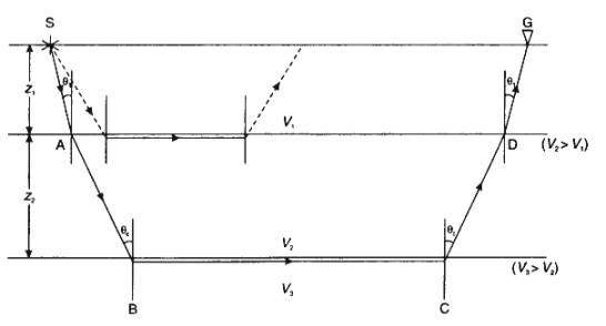
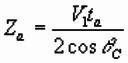
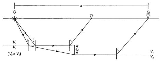
Planar Interfaces: Two Layers

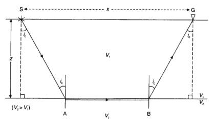
For critical refraction at top of second layer, total travel time from source S to receiver G is given by:

Hypoteneuse and horizontal side of end 90^o-triangle are:

and respectively.

So, as two end triangles are the same:

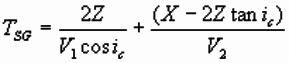
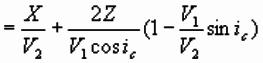
At critical angle, Snell’s law becomes:

Substituting for V₁/ V₂, and using cos²q + sin²q = 1:

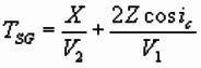
This equation represents a straight line of slope 1/V₂ and intercept

Interpretation of Two Layer Case

From traveltimes of direct arrival and critical refraction, we can find velocities of two layers and depth to interface:

1. Velocity of layer 1 given by slope of direct arrival

2. Velocity of layer 2 given by slope of critical refraction

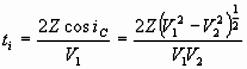
3. Estimate t_i from plot and solve for Z:

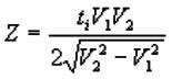
Depth from Crossover Distance

At crossover point, traveltime of direct and refraction are equal:

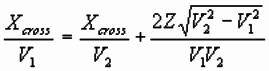
Solve for Z to get:

[Depth to interface is always less than half the crossover distance]

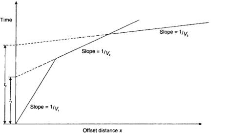
Planar Interfaces: Three Layer Case

In same way as for 2-layer case, can consider triangles at ends of raypath, to get expression for traveltime.

After simplification as before:

The cosine functions can be expressed in terms of velocities using Snell’s law along raypath of the critical refraction:

Again traveltime equation is a straight line, with slope 1/V₃ and intercept time t₂.

Warning:

q₁ is NOT the critical angle for refraction at the first interface.

It is an angle of incidence along a completely different raypath!

Interpretation of Three Layer Case

In three layer case, the arrivals are:

1. Direct arrival in first layer

2. Critical refraction at top of seconds layer

3. Critical refraction at top of third layer

Because, intercept time of traveltime curve from third layer is a function of the two overlying layer thicknesses, we must solve for these first.

Use a layer-stripping approach:

1. Solve two-layer case using direct arrival and critical refraction from second layer to get thickness of first layer.

2. Solve for thickness of second layer using all three velocities and thickness of first layer just calculated.

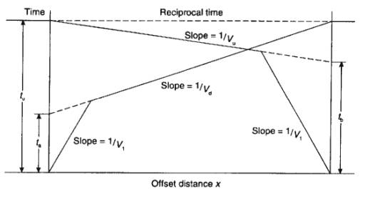
Planar Interfaces: Multi-Layer Case

For a subsurface of many plane horizontal layers, the planar interface travel time equation can be generalised to:

where q_i is the angle of incidence at the ith interface, which lies at depth Z_i at the base of a layer of velocity V_i.

Interpretation

Proceeds by a layer-stripping approach, solving two-layer, three-layer, four-layer etc. cases in turn.

Dipping Planar Interfaces

When a refractor dips, the slope of the traveltime curve does not represent the "true" layer velocity:

• shooting updip, i.e. geophones are on updip side of shot, apparent refractor velocity is higher

• shooting downdip apparent velocity is lower

To determine both the layer velocity and the interface dip, forward and reverse refraction profiles must be acquired.

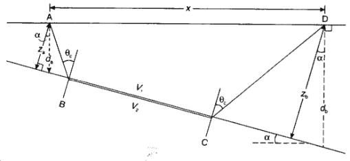
Note: Travel times are equal in forward and reverse directions for switched, reciprocal, source/receiver positions.

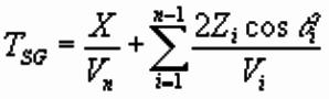
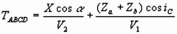
Dipping Planar Interface: Two Layer Case

Geometry is same as flat 2-layer case, but rotated through a, with extra time delay at D. So traveltime is:

Formulae for up/downdip times are (not proved here):

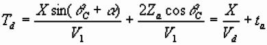
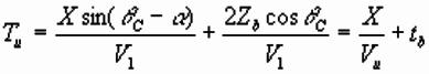
where V_u/ V_d and t_u/ t_d are the apparent refractor velocities and intercept times.

;

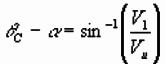
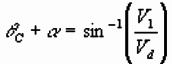
Can now solve for dip, depth and velocities:

1) Adding and subtracting, we can solve for interface dip a and critical angle q_C:

;

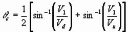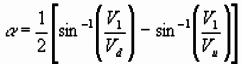
[V₁ is known from direct arrival, and V_u and V_d are estimated from the refraction traveltime curves]

2) Can find layer 2 velocity from Snell’s law: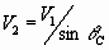

1. Can get slant interface depth from intercept times, and convert to vertical depth at source position:

;

Faulted Planar Interface

If refractor faulted, then there will be a sharp offset in the travel time curve:

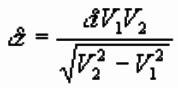
Can estimate throw on fault from offset in curves, i.e. difference between two intercept times, from simple formula:

Interpretation of Realistic Traveltime Data

With field data it is necessary to examine traveltime curves carefully to decide on best method to use:

• How many refraction branches are there, i.e. how many layers?
• Are anomalous times due to mispicking or real?
• Small anomalies can be ignored, but larger ones require other methods, e.g. Plus-Minus.
• Multiple source positions allow, some inference of depth of anomaly: near-surface anomalies align

Surface Topography Intervening Velocity Anomaly

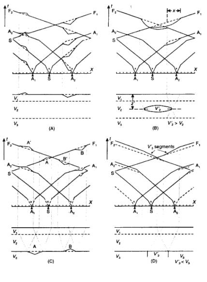
Refractor Topography Refractor Velocity Variation

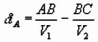
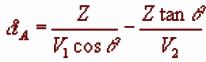
Delay Times

For irregular traveltime curves, e.g. due to bedrock topography or glacial fill, much analysis is based on delay times.

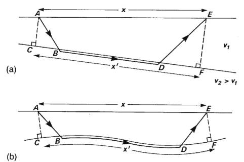
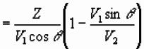
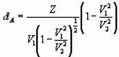
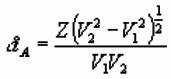
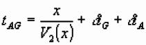
Total Delay Time

Difference in traveltime along actual raypath and projection of raypath along refracting interface:

;

Total delay time is delay time at shot plus delay time at geophone:

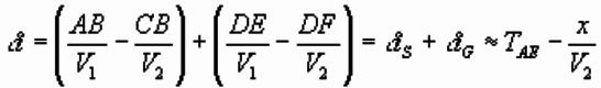
For small dips, can assume x=x^I and:

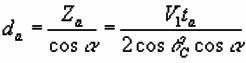
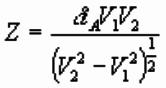
Refractor Depth from Delay Time

If velocities of both layers are known, then refractor depth at point A can be calculated from delay time at point A:

Using RH triangle to get lengths in terms of z:

Using Snell’s law to express angles in terms of velocities:

Simplifying:

So refractor depth at A is:

Varying Interface & Refractor Velocity: Plus-Minus Method

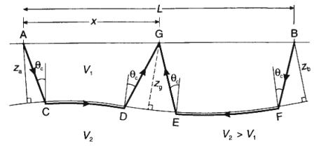
Hagedoorn’s Plus-Minus method used for more complex cases:

• Undulating interfaces
• Changes in refractor velocity along the profile

Plus-Minus:

• Requires forward and reverse travel times at geophone location to find delay time and refractor velocity at geophone
• Assumes interface is planar between D and E, can result in smoothing of actual topography
• Assumes dips less than ~10^o.

Delay time at G given by:

which can be found from observed data.

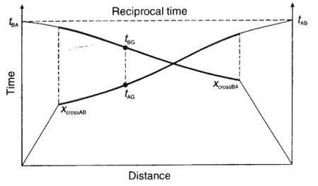
Plus and Minus Terms

Using previous figure can write down forward/ reverse traveltimes:

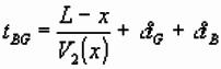
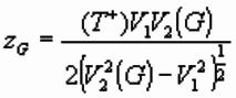
Minus Term

Used to determine laterally varying refractor velocity, i.e. V₂(x):

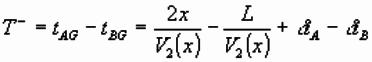
• Velocity given by local slope of plot of (T^-) vs. x, distance along profile. Note factor of 2 compared with the plane layer method.

• Velocity may change along profile, so written as V₂(x). Different values of V₂ can be used for calculation of interface depth using Plus term

Plus Term

Determines refractor depth at a location from delay time there:

So from delay time formula for depth, depth at G given by:

• Depth can be determined at each geophone location where forward and reverse traveltimes recorded using V₂ estimated for that position

Plot of Minus Term

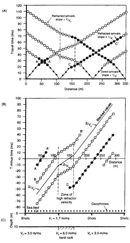
A. Composite traveltime distance plots for four different shots

B. Plot of Minus Terms: note lateral changes in refractor velocity

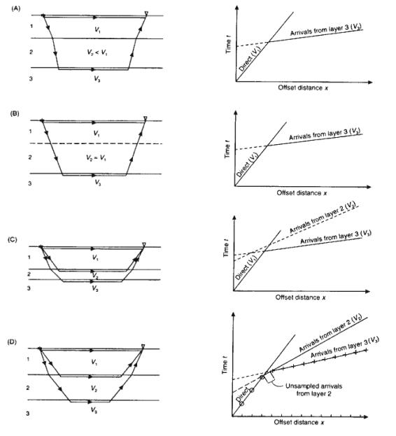
Hidden Layer Problem

Layers may not be detected by first arrival analysis:

A. Velocity inversion produces no critical refraction from layer 2

B. Insufficient velocity contrast makes refraction difficult to identify

C.Refraction from thin layer does not become first arrival

D.Geophone spacing too large to identify second refraction

Seismic Refraction Energy Sources

Source for a seismic survey source has to be chosen bearing in mind the possible signal attenuation that can occur, often a function of the geology.

Requirements

• Sufficient energy to generate a measurable signal at receiver

• Short duration pulse, i.e. containing enough high frequencies, to resolve the desired subsurface layering

• Repeatable source with a known, consistent waveform

• Minimal mechanical noise

• Ease of operation

There are many different seismic refraction sources, but the most important are:

On land:

sledge hammer, weight drop, shotgun (shallow work)

dynamite (crustal studies)

At sea:

airgun (oil exploration, crustal studies)

Land Seismic Sources: Mechanical

Sledge Hammer

A sledge hammer is struck against a metal plate:

• Vertically down on plate to generate P waves
• Horizontally against side of plate to produce S waves

Inertial switch on hammer triggers data recording on impact.

• Problems with repeatability and possible bouncing of hammer.
• Used for refraction spreads up to 200 m.

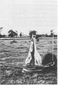
Accelerated weight–drop

Mechanical system, using compressed air or thick elastic slings, forces weight onto baseplate with greater force

• Better repeatability than sledge hammer

Land Seismic Sources: Explosive

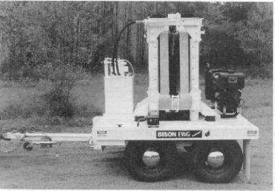
Buffalo Gun

Metal pipe inserted up to 1 m into the ground, and a blank shotgun cartridge fired.

Exploding gases from gun impact ground and generate the seismic pulse.

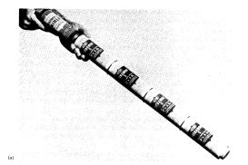
Dynamite

Shot holes up to 30 m are drilled, and loaded with dynamite, which usually comes in 0.5 m plastic cylinders that can be screwed together.

Marine Seismic Sources: Airgun

Airguns are most common seismic source used at sea.

Essentially, an airgun is a cylinder that is filled with compressed air, and then releases the air into the water.

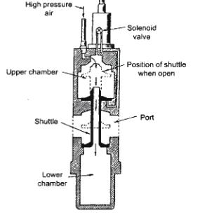
The sudden release of air creates a sharp pressure impulse in the water.

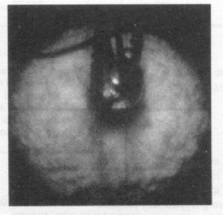
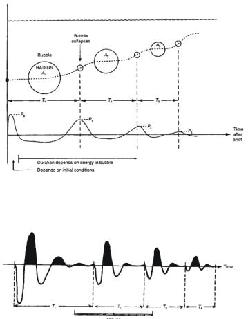
Airgun Bubble Oscillation

1. Air bubble from airgun expands until pressure of surrounding water overcomes its expansion, and forces it to contract.

2. Bubble then collapses, compressing the air until the air pressure exceeds the water pressure, and the bubble can expand again.

3. Expansion and collapse continues as bubble rises to surface, giving oscillatory signal characteristic of single airgun.

• Airguns are usually deployed at a depth of a few metres, so there is always a reflection from sea surface, called the ghost.

• The sea surface RC is –1, so ghost is almost as strong as original signal, producing a trough-peak response.

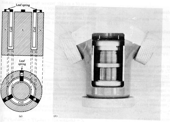
Land Sensor: The Geophone

Geophone is essentially only type of sensor used on land.

A geophone comprises a coil suspended from springs inside a magnet.

When the ground vibrates in response to a passing seismic wave, the coil moves inside the magnet, producing a voltage, and thus a current, in the coil by induction.

• As coil can only move in one direction, usually vertical, the geophone only senses the component of seismic motion along axis of coil.

• Three orthogonal geophones necessary to fully characterise seismic ground motion.

• Geophones respond to the rate of movement of the ground, i.e. particle velocity, and are often laid in arrays of several phones.

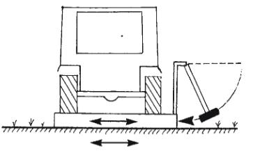
Principle of Geophone

Geophone Damping

As geophone coil moves inside magnet, current induced in coil produces a magnetic field that opposes, i.e. damps, the movement of the coil.

• If a geophone is tapped, the oscillation of coil will die out.

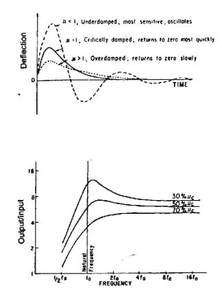
• At critical damping, coil will return to rest most quickly.
• If damping very small, coil will oscillate at the natural frequency of the electromechanical system.
• Normal damping is 70% critical.

Natural Frequency

Natural frequency and damping affect the range of frequencies the geophone can record:

• 14 Hz geophones used in oil exploration
• 30 Hz geophones used in high resolution studies
• 100 Hz geophones used in very shallow work

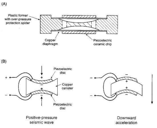
Marine Sensor: The Hydrophone

Hydrophones used to detect the pressure variations in water due to a passing seismic wave.

A hydrophone comprises two piezoelectric ceramic discs cemented to a sealed hollow canister.

• A pressure wave squeezes the canister, bending the ceramic and generating a voltage.

• The two discs are connected in series so that the output generated by acceleration of the hydrophone cancels

• Pressure will squeeze ceramics and so produce output.

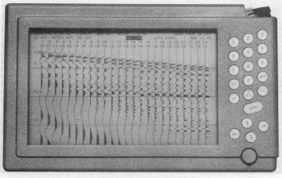
Recording Instruments

Electrical output from geophone, i.e. voltage, is digitised by recording instrumentation and written onto tape or disk.

Data are viewed on monitor records in field to check quality.

Many different type of recording instrument available.

Example (Strataview, Geometrics)

Face of a Strataview seismograph commonly used in shallow seismic work, and able to record up to 24 channels.

Recording Channel

Channel refers to electrical input to recording system. Might be from a single geophone as in engineering work, or a group of 9 geophones, common in oil exploration.

• In oil exploration work, recording systems can record up to 8000 channels.

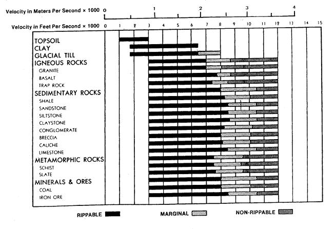
Application to Assessment of Rock Quality

Seismic refraction most commonly employed where velocities increase suddenly with depth, e.g. determining depth to bedrock.

From the estimated layer velocities estimates of rock strength and excavation difficulty can be made.

• Rippability is ease with which ground can be excavated with a mechanical digger, varies with tractor size and power.

• In 1958, the Caterpiller Tractor Company began using seismic velocities from refraction experiments to estimate rippability.

Rippability for various common rocks:

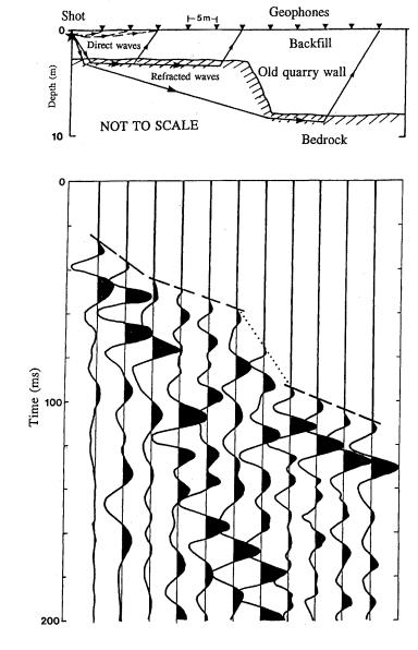
Application to Landfill Investigation 1

Seismic methods rarely used in landfills, because seismic waves are often attenuated in the unconsolidated materials.

• Most landfills comprise hole excavated into bedrock, filled with waste, and covered by an impermeable compacted clay cap.
• Gases are then vented in a controlled fashion through outlets.

Fault analysis used to find quarry height from offset in intercepts

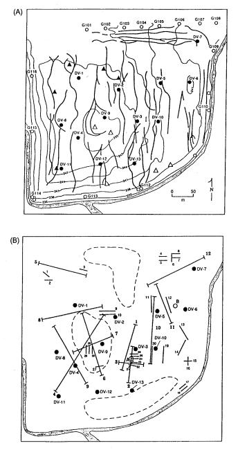
Application to Landfill Investigation 2

Integrity of clay cap from refraction velocities

• Low P wave velocities used to identify fractures in the clay cap that required repair.
• P wave velocities in the fractured zones were around 370 m/s, compared with 740 m/s over unfractured areas.
• In some areas, not possible to obtain critical refraction due to velocity in the fill being lower than in clay cap.

Application to Tectonics: Structure of Ocean Crust

Fracture zones comprise active transform faults located between the ends of spreading segments on a midocean ridge, plus their lateral extension

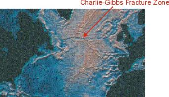
Fracture zones contain some of the most rugged topography on Earth

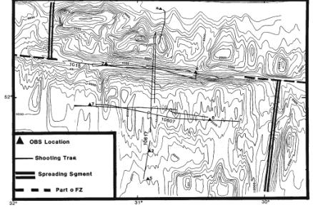
Crustal thickness can be measured by firing explosive shots over seafloor deployed ocean-bottom

• Crustal refraction data usually plotted using reduced travel time, i.e. a linear time shift.

• If vertical axis is T-X/8000, a refraction with velocity of 8000 m s^-1 will appear horizontal

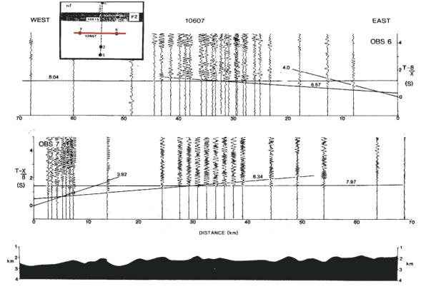
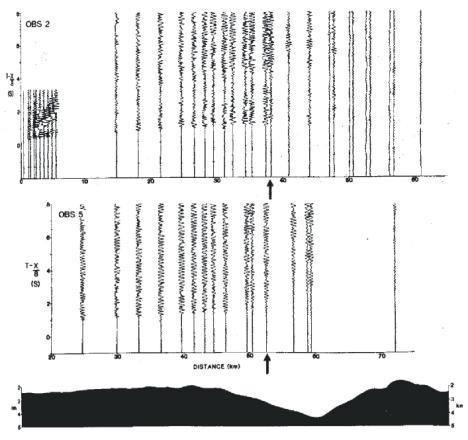
Reversed Refraction Profiles over Normal Ocean Crust

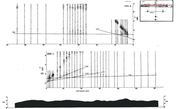
Reversed Refraction Profiles along Fracture Zone

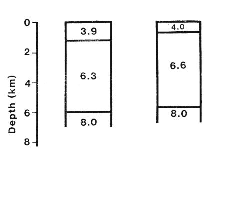
Plane Layer Solution for Normal Ocean Crust

OBS 7 OBS 6

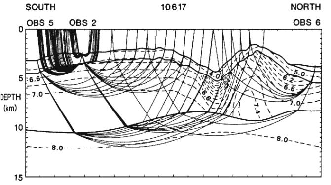
Plane Layer Solution for Normal Fracture Zone Crust

OBS 2 OBS 6

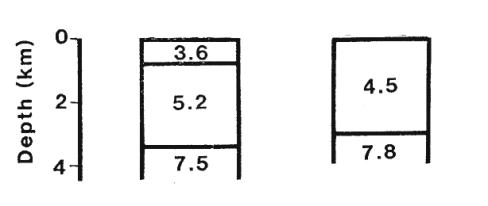
Fracture zone crust is thin and has low velocities due to fracturing and hydrothermal circulation

Refraction Profile Orthogonal to Fracture Zone

Raytracing for Large Lateral Velocity Variations